
In this article, I will talk about TinyML, a fast-growing field of Machine Learning (ML). The article starts with a brief background, followed by TinyML's definition, benefits, applications, and challenges. After that, I will discuss how we implement TinyML and conclude the article by discussing some use cases.
Background
This section briefly discusses some background needed for the article.
Artificial Intelligence
Artificial intelligence (AI) refers to the theoretical and practical application of computer systems to execute functions traditionally needing human intellect, including speech recognition, decision-making, and pattern recognition.
Machine Learning
Machine Learning (ML), a subfield of AI, employs algorithms trained on data to develop self-learning models that are capable of predicting results and classifying data without human intervention
Deep Learning
Deep Learning (DL), a subfield of ML, uses Neural Networks (NNs) to extract patterns from data. An NN consists of interconnected nodes, called neurons. A neuron is a computational unit that processes input data and generates an output. Those nodes are organized in layers, as in Figure 1. The connections (a.k.a synapses) between nodes are called weights, or parameters. The output of a neuron is computed by multiplying each input by its respective weight, summing these products, and subsequently applying a non-linear function known as the activation function.

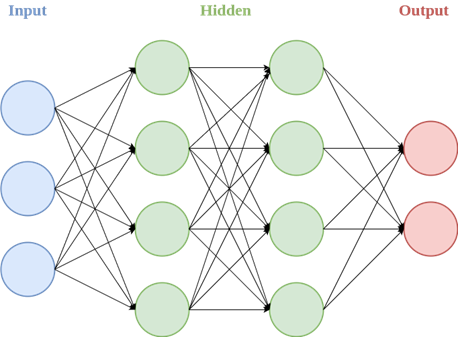
Figure 1: Left: a neuron. Right: a NN with an input layer, 2 hidden layers, and an output layer.
Convolution Neural Network
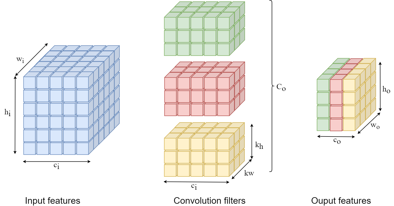
Convolutional Neural Network (CNN) is a type of NN used for processing data with grid-like topology, like images. The basic element of a CNN is the convolution operation, where a convolution filter is applied to an input of n channels to produce one channel of the output. Figure 2 shows an example of applying 3 filters of co33 dimension to an input of ci hiwi dimension to produce an output of co howodimension.
What is TinyML?
Tiny machine learning (TinyML) is a fast-growing field of machine learning technologies and applications, including algorithms, hardware, and software that are capable of performing sensor data analytics directly on devices using minimal power. This capability enables continuous machine-learning operations on devices powered by batteries.
Benefits
Applying TinyML algorithms on devices, where data is generated, brings many benefits including:
- Mitigating bandwidth limitations: Running TinyML models locally allows IoT devices to function without the need for constant Internet connectivity.
- Reducing latency: Local execution of TinyML models eliminates the delays associated with data transmission to the Cloud.
- Improving privacy and security: Processing data on-device enhances user privacy and security by avoiding data transmission to the Cloud.
- Low energy consumption: Minimizing data transmission reduces energy use, extending the battery life of IoT devices.
- Reducing cost: Local data processing decreases costs related to network data transmission and Cloud processing.
- Reliability: Reducing dependency on network connectivity improves the reliability of IoT systems.
Applications
TinyML can be applied in different applications including:
- Personalized Healthcare: TinyML enables wearable devices, like smartwatches, to persistently monitor user activities and oxygen levels, offering tailored health suggestions.
- Smart Home: TinyML facilitates object detection, image recognition, and face detection on IoT devices, to create intelligent environments, like smart homes and hospitals.
- Human-Machine Interface: TinyML enables applications in human-machine interfaces, such as recognizing hand gestures and interpreting sign language.
- Smart Vehicle and Transportation: TinyML is capable of executing object detection, lane detection, and making decisions without an Internet connection, ensuring quick response times in autonomous driving environments.
- Predictive Maintenance: In predictive maintenance, TinyML models predict when equipment is likely to fail and allow preventive maintenance before the equipment fails, which reduces unplanned downtime.
Challenges
TinyML is a composition of Embedded systems and ML. Embedded hardware is extremely limited in computation power, memory, and storage. For example, Arduino Nano 33 BLE Sense has the following specifications:
- Clock speed: 64MHz.
- Storage: 1MB.
- Memory: 256KB.
Conversely, today’s ML models are big and need a high computation power. For example, MobileNetV2, which Google built to fit mobiles, is 13.6 MB and needs 6.8 MB of memory, which is impossible to deploy on an Embedded system like Arduino Nano 33 BLE Sense.
TinyML Approaches
There are two main approaches to implementing TinyML: going from big to tiny or starting tiny. Going from big to tiny, including:
- Pruning.
- Quantization.
Starting tiny, including:
- Efficient Architectures.
- Neural Architecture Search (NAS).
The following sub-sections discuss those approaches briefly.
Pruning
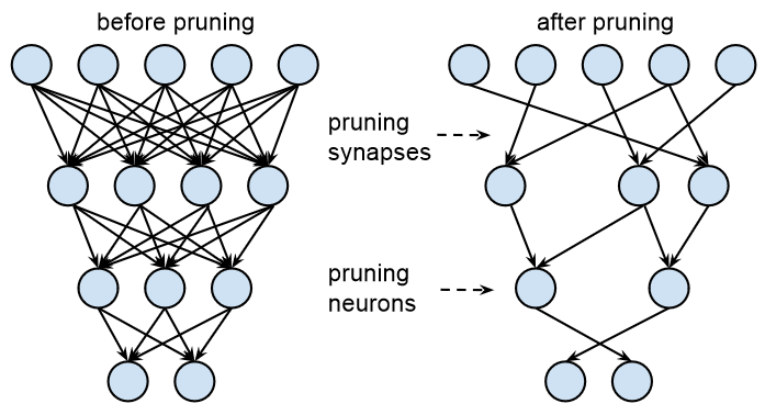
Pruning means turning off, a node or weight by setting its value to zero. The goal of pruning is to reduce the number of parameters, which reduces a model’s size and improves computation efficiency. The result of pruning is a sparse model (compared to an un-pruned dense model), where sparsity is defined as Number of pruned parametersTotal number of parameters. Figure 3 shows a NN before and after pruning.
Normally, pruning is applied in an iterative process where in each iteration, a portion of the NN is pruned and then followed by a fine-tuning, as shown in Figure 4. The process ends when the required sparsity or the target quality metric (e.g., accuracy) is met.

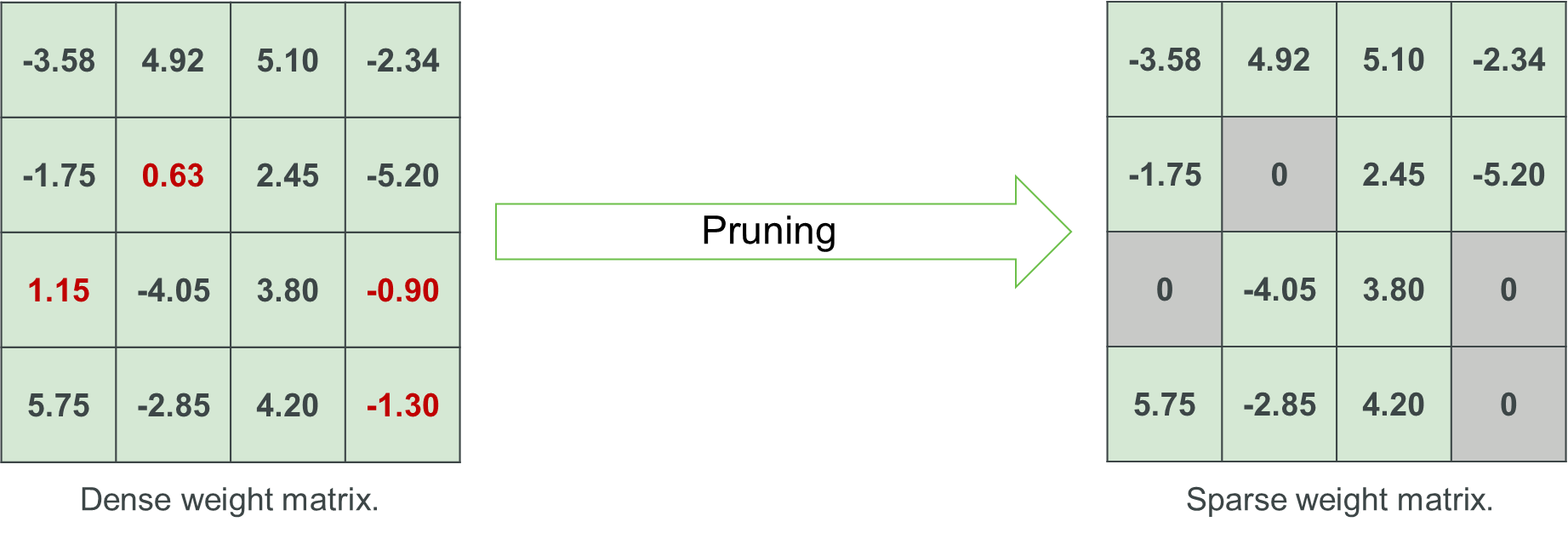
Example
The following is an example of pruning a 4 x 4 weight matrix, the sparsity ratio is 25% (i.e., 25% of the parameters has been set to zero).
Quantization
Quantization is the process of mapping input values from a continuous set to a discrete set. The difference between the input value and the quantized value is the quantization error. In neural networks, weights and activations are normally in 32-bit floating point values. By using quantization, precision can be reduced to a lower-precision datatype, such as 8-bit fixed point integers. This helps reduce the size of a model and the inference latency.
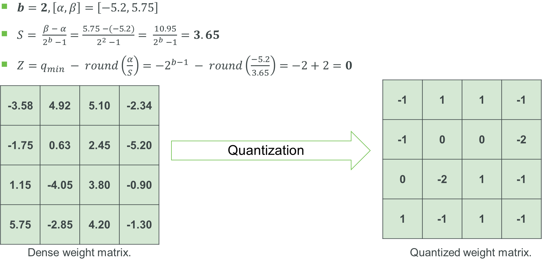
Example
The following is an example of quantizing a 4 x 4 weight matrix using 2 bit.
Efficient Architectures
Efficient architectures consist of efficient building blocks, designed from scratch, and used in building CNN models. For example, Figure 2 shows an example of applying what is called standard convolution, however, this is not the only type of convolution. The researchers in Xception introduced a new, more efficient, convolution operation called depthwise separable convolution as shown in Figure 5.
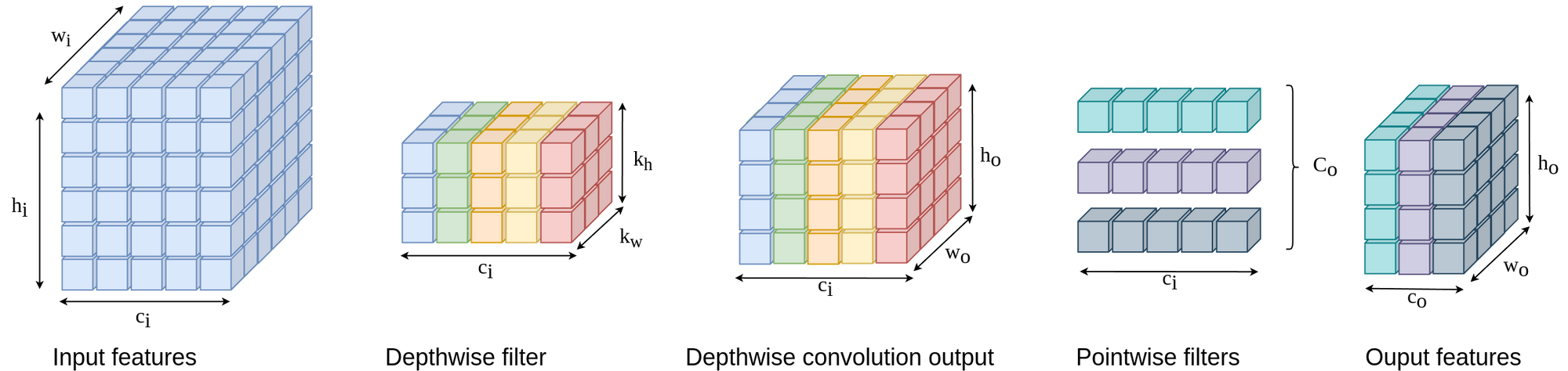
The example shown in Figure 5 needs (3 x 3 x 5) x 1 + (5 x 3) = 60 parameters to produce the same number of nodes as in Figure 2, where the conventional convolution needs (3 x 3 x 5) x 3 = 135 parameters.
Neural Architecture Search (NAS)
In designing NNs, different design-related decisions must be taken. For example, in CNNs such decisions include determining:
- The number of layers, and channels (i.e., filters).
- The size of convolution kernels.
- The input resolution.
Efficiency metrics, e.g., latency, model size, and accuracy, should be considered as well. This implies that the design space is very large, for example, the number of sub-networks in the Once-for-All (OFA) design space is > 1019. It’s impractical to manually search for an efficient architecture.
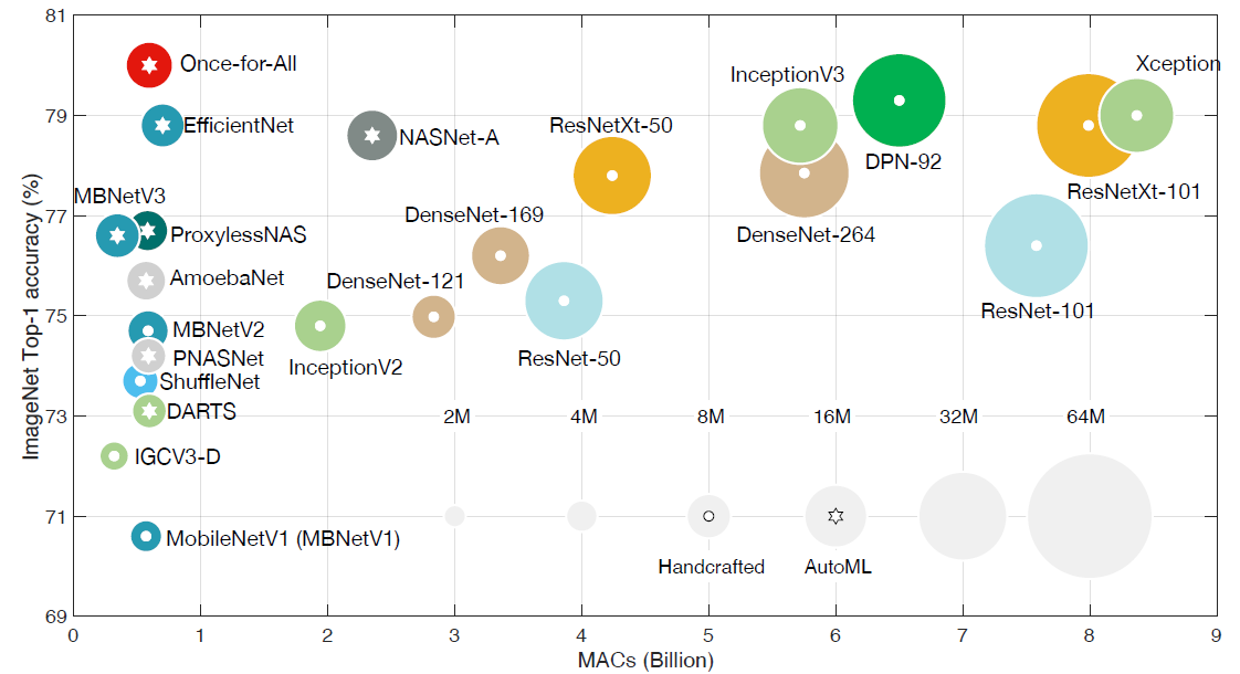
However, the use of Neural Architecture Search (NAS) enables the automation of the search process. Recently, the use of NAS has become popular for designing efficient models as shown in Figure 6.
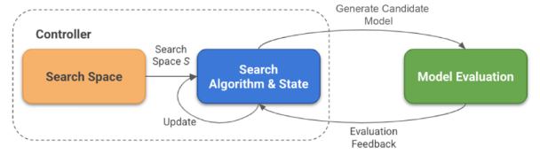
NAS components:
A NAS consists of the following main components:
- Search Space: The search space defines the set of architectures that can be built.
- Search Strategy: The search strategy defines how the search space is explored.
- Performance Estimation Strategy: The performance estimation strategy evaluates the fitness of the candidate architecture.
Figure 7 shows the NAS's main components:
Conclusion
In this article we discussed TinyML, what it means, its benefits, challenges, and applications. We also talked about the main approaches used to produce TinyML models.
References
- Tiny Machine Learning (TinyML): https://www.edx.org/certificates/professional-certificate/harvardx-tiny-machine-learning.
- Gaurav Menghani. Efficient Deep Learning: A Survey on Making Deep Learning Models Smaller, Faster, and Better. ACM Computing Surveys, 55(12):1–37, March 2023.